The SOE Project: Part 2

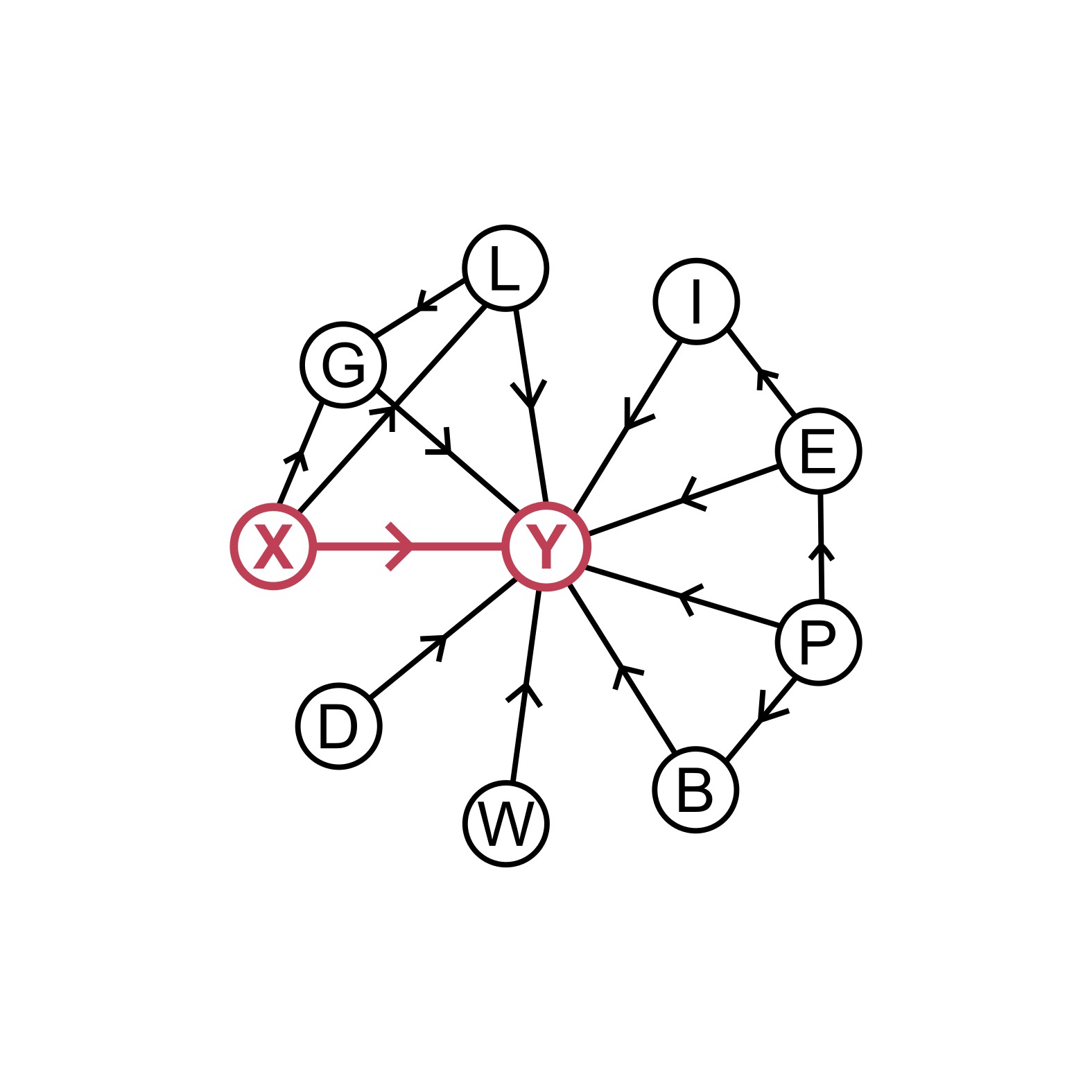
As outlined in part 1 of this series, during an SOE, the government of TnT has the special power to detain a criminal using a preventative detention order (PDO). The government uses PDOs to disrupt criminal networks, decreasing their ability to commit violent crime. If this theory were true, then the execution of a preventative detention order in a community (the independent variable, \(X\)) should cause a reduction in violent crime in the surrounding community (the dependent variable, \(Y\)). The effects of detentions are expected to be localised to a community, particularly because most gangs in TnT are small and community-based ^[4][6]. Additionally, I expect that the effects of a PDO will only be temporary because criminal networks/gangs can adapt to the disruption.

I also expect that the rate of violent crime, \(Y\), will be influenced by a host of other factors such as:

• Beliefs, \(B\)
• Disruptions (pandemics, holidays, etc), \(D\)
• Economic Indicators, \(E\)
• Gang Prevalence / Strength, \(G\)
• Infrastructure, \(I\)
• Perceived Legal Consequences, \(L\)
• Population Demographics, \(P\)
• Weather, \(W\)

The graph, representing my causal model, shows how I expect these factors to be related. In the graph \(X → Y\) means that \(X\) (the government executing a PDO in a community) somehow directly affects \(Y\) (the rate of violent crime in that community). Though my goal is to determine how \(X\) affects \(Y\), as shown in the graph, I expect there to be many interesting relationships between the factors. This will complicate the analysis.

Assumption 1: The error term has a mean of zero.

Given the current model specification, the error term, \(\epsilon\), can not have a mean of zero because I have not accounted for the baseline violent crime rate throughout the country. In the current setup, \(\epsilon\) subsumes the baseline crime rate. This issue could be solved by including a constant factor, \(c\). A single constant factor, however, would overlook the fact that crime rates vary throughout the country and from week-to-week.

The best solution would be to use two-way fixed effects, \(\alpha_i\) and \(\lambda_t\). \(\alpha_i\) would represent the baseline crime rate in geographic area \(i\) over the period of the study, whereas \(\lambda_t\) would represent the baseline crime rate during week \(t\) across the entire country. These two-way fixed effects thereby allow the statistical model to center its errors around the mean of zero ^[2].

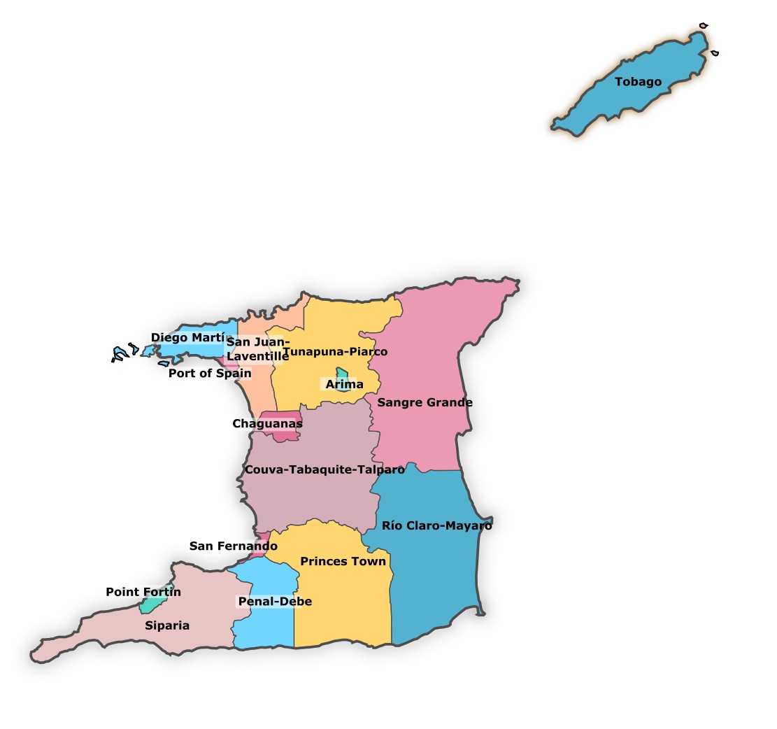
To accommodate these two way fixed effects, I will have to disaggregate the data to geographic subdivisions that make up the country such as cities or police administrative zones. The regression equation now becomes:

\[\begin{align*} Y_{i,t} = &\beta_1 X_{i,t} + \beta_2 B_{i,t} + \beta_3 D_{i,t} + \beta_4 E_{i,t} \\ &+ \beta_5 G_{i,t} + \beta_6 I_{i,t} + \beta_7 L_{i,t} + \beta_8 P_{i,t} \\ &+ \beta_9 W_{i,t} + \alpha_i + \lambda_t + \epsilon \end{align*}\]

Assumption 2: The regression model is linear.

The regression model is nonlinear because \(Y_{i,t}\) is not a continuous variable nor can it be determined by a linear combination of the current independent variables. Firstly, the rate of violent crime in a given week, \(Y_{i,t}\), is non-negative and discrete. Half a murder cannot happen or be taken away. Secondly, as each row of data now represents geographic subdivisions rather than the entire country, a lot of the \(Y_{i,t}\) variables will equal zero simply because no crime occurred in that region during the time frame under consideration. This will skew the data so that it is non-linear. To account for these first two issues I will use a non-OLS method, and one designed particularly to study discrete data such as \(Y_{i,t}\). The poisson, negative binomial, and pseudo-poisson maximum likelihood (PPML) methods are suitable techniques for discrete data ^[1][8].

A third issue is that by considering geographic subdivisions rather than the country as a whole, I unknowingly made the assumption that variables in neighbouring regions do not affect the rate of violent crime in the region under consideration. This is wrong. Though I assume criminals in the largely community based gangs of TnT commit crime within their community, they may still cross the geographic borders that I specify to do so. I account for this issue by introducing a new spillover variable, \(S\), that will measure the number of PDOs executed in neighbouring geographic regions.

Lastly, \(Y_{i,t}\) is unlikely to be expressed as a linear combination of its current variables because the effect of a PDO is unlikely to be felt immediately. In reality, this effect may be felt in the following week or even month. I account for this issue by including lags of the variables in the preceding periods. Where \(A\) represents some variable, let \(A'_t\) be a vector of lags of \(A\) up to period \(t\) for some given number of lags \(j\). \(A'_t=(A_t, A_{t-1},..., A_{t-j})\). Similarly \(\beta'\) is a vector of coefficients that correspond to each lead. The new regression equation becomes:

\[\begin{align*} Y_{i,t} = &\beta'_1 X'_{i,t} + \beta'_2 S'_{i,t} + \beta'_3 B'_{i,t} + \beta'_4 D'_{i,t} \\ &+ \beta'_5 E'_{i,t} + \beta'_6 G'_{i,t} + \beta'_7 I'_{i,t} + \beta'_8 L'_{i,t} \\ &+ \beta'_9 P'_{i,t} + \beta'_{10} W'_{i,t} + \alpha_i + \lambda_t + \epsilon \end{align*}\]

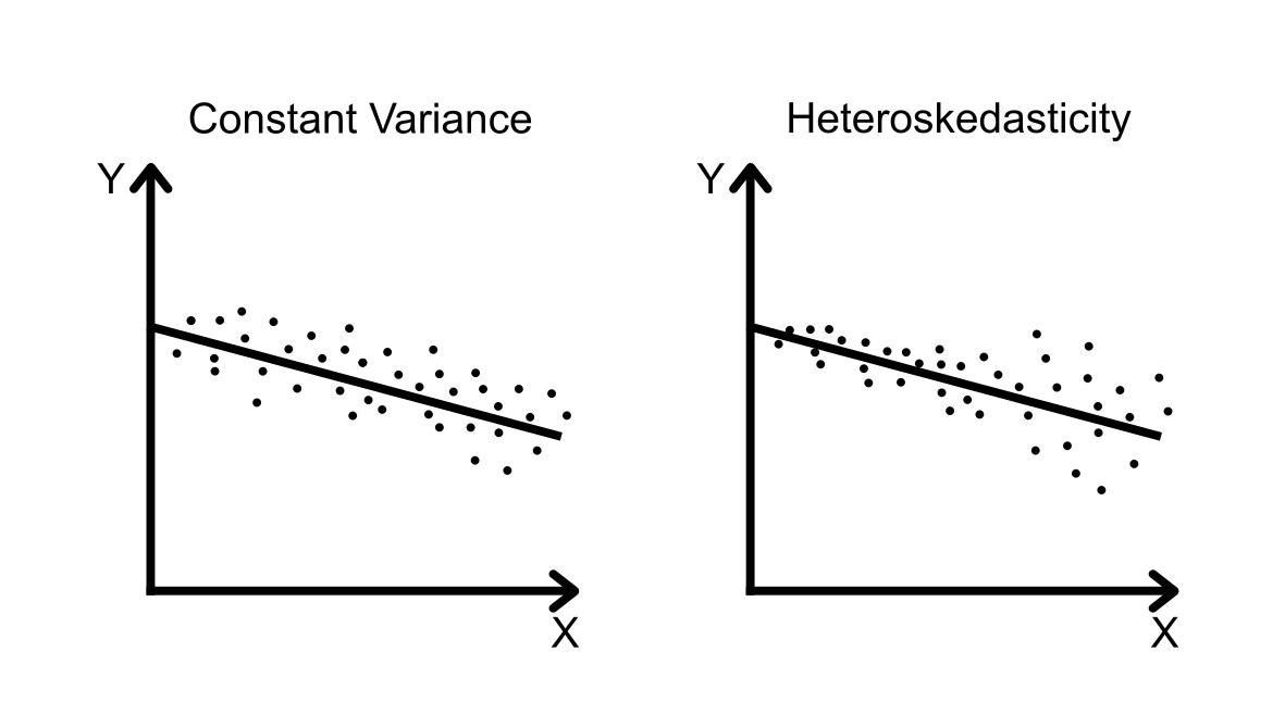
Assumptions 6 & 7: The error terms have a constant variance and are normally distributed.

The error terms are not expected to have constant variance or be normally distributed. As discussed under assumption 2, \(Y_{i,t}\) will frequently equal zero, skewing the data away from a normal distribution. Secondly, it is possible that the government will execute more PDOs in areas with more resilient criminal networks, as it is harder for them to identify the key criminal actors. Due to the resilience of these networks, the execution of any individual PDO may have less effect on crime rates, leading to an increase in the variance of outcomes. Thus the error terms may have a non-constant variance with respect to \(X_{i,t}\).

Both of these issues will be addressed by statistically modeling the data using the PPML method as mentioned under assumption 2. Unlike the negative binomial regression techniques, the PPML method naturally accounts for zero-bias and heteroskedasticity (non-constant variance) ^[8].